 Quantitative terms, such as the maximum difference in dB, are also problematic. For example, a 10 dB difference in interference when levels are at -90 dB is very different from one when levels are at -20 dB. Furthermore, is comparing magnitude sufficient, or should both magnitude and phase be considered? Later in this article, two different quantitative methods for comparing datasets are applied to the following example.
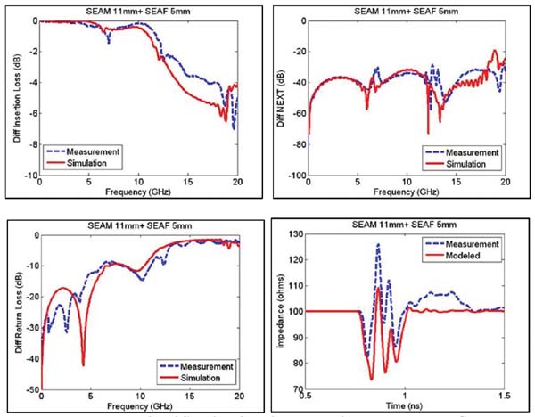
To begin the correlation discussion, consider the measured and simulated performance of a high-density 16 mm mezzanine connector. The simulated response was generated using a full-wavelength modeling tool. Care was taken to ensure sufficient mesh density and port configuration protocols were followed using nominal dielectric material characteristics. The measured response includes the connector and its size. Onboard TRL/M calibration structures were used to calibrate the VNA and de-embed measurement effects in the apparatus. Care was taken to ensure that the measured size exactly matches the simulated size. The results are shown in Figure 15. Comparing the responses in Figure 15, the correlation is generally within expectations. The impedance profile shown in Figure 15 was generated from the measured/simulated touchstone files using time-domain convolution.
Intel publicly released a document on the quality of the connector model in September 2011 [2]. This document introduces the concept of Model Quality Factor, as a means of measuring the accuracy of a simulation-based model compared to its measured performance where it operates, when:

xx = x
xx = Model Quality Factor for impedance, insertion loss, and interference
x1 = reference area
x2 = area between the measured and simulated curves.
A large positive MQF value indicates a high degree of correlation.
A small (or negative) MQF value indicates a relatively poor correlation. The method is based on calculation areas in the time-domain graphs. This method was applied to the results shown in Figure 15 for a 16 mm mezzanine connector. The first step in the MQF calculation is to transform the S-parameter connector model and measurements into time-domain graphs. This was done using Agilent ADS2.011.05.
The MQF for impedance was calculated to be -0.15, indicating a relatively poor correlation. This is due to a low simulated impedance compared to the measured value.
Figure 16 illustrates the area calculation in the MQF calculation. Note that the MQF span is limited to the connector region or twice the connector propagation time on an impedance-time graph. The MQF impedance does not specify the rise time; however, the rise time affects the MQF. Figure 16 had a rise time of 30 ps (20–80%), resulting in an MQF of -0.15. At a rise time of 50 ps, the MQF degraded to -0.28, and at 100 ps, the MQF dropped to -0.6.

The MQF insertion loss is based on the Time Domain Transmission (TDT) response. Rise Time Degradation, or TDT, is equivalent to the supplied insertion loss when the source rise time is defined. The MQF for insertion loss was calculated to be 0.43, and the corresponding analysis is shown in Figure 17.

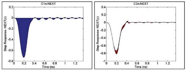
MQF (NEXT) interference is also based on the DTT (Time Domain Transmission) response. Time Domain NEXT also depends on the source rise time, which is not specified. The MQF for NEXT was calculated to be 0.85, and the corresponding analysis is shown in Figure 18.
6]. FSV has an advantage over MQF in that it can be applied to either time-domain or frequency-domain datasets. MQF has the advantage of being much simpler to implement if we write original code. FSV results in a qualitative value ranging from excellent to poor. This assigns quantitative FSV values from <0.1 (excellent) to >1.6 (poor). FSV considers the absolute difference between two datasets and conditions as the Amplitude Difference Measure (ADM). For example, achieving good correlation across a broad spectrum with a fairly constant dependent variable would be presented as a low ADM. FSV also considers differences in the features of two datasets, calculated as the first derivative of the data to accentuate changes in the curves. This is known as the Feature Difference Measure (FDM). For example, good connector resonance correlation would be shown as a low FDM value.

The geometric mean of the ADM and FDM is combined to form the Global Difference Measure (GDM). GDM can be considered the overall correlation between two datasets. ADM, FDM, and GDM can be plotted over the independent variable to indicate where the models are similar or different. It is also common to plot the histogram to show what percentages of data points are well correlated. The histogram is divided into six categories, with quantitative terms assigned to the qualitative categories of the histogram.

The FSV application is available for download at www.upd.edu/web/gcem [6] and was used to create Figures 19-21. Figure 19 shows that the measured and simulated insertion loss datasets had “very good” correlation based on the GDMtot value of 0.13. GDMtot is essentially a “rating number,” which includes the amplitude and function differences in the datasets.
Figure 20 shows the measured and simulated NEXT datasets that had “good” correlation based on the GDMtot value of 0.3. As with the insertion loss data, both ADM and FDM showed better correlation than the geometric mean.
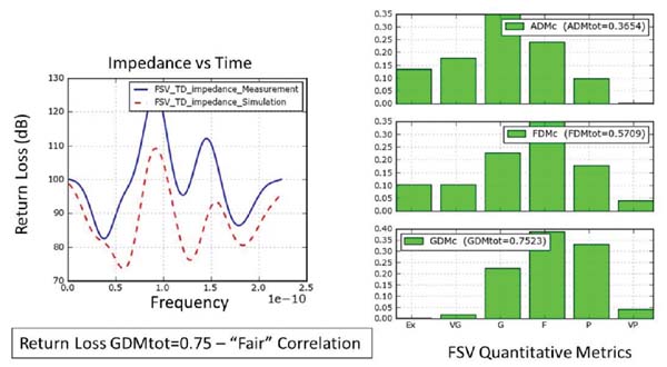
Figure 21 shows that the measured and simulated impedance datasets had “fair” correlation based on the value of 0.75 GDMtot.
Conclusions and Recommendations:
Validating high-speed, multi-pin connectors has proven challenging, as imperfect fitting testing significantly impacts the results. On the measurement side, accurate onboard calibration standards are necessary for consistent de-embedding. On the simulation side, connector material parameters are estimates, and the model's mesh density can affect the results. It is critical that the measured size be included in the simulation, as even minor size differences will lead to variations between the measurement and simulation results.
Two different model quality metrics were applied to the measurement and simulation of the connector's differential S-parameters. These metrics are required for this type of model, and achieving a very good correlation is challenging given the complexity of microwave structures.
The transmission parameters (IL and NEXT) tend to show better correlation compared to the reflection parameters (RL and impedance). The qualitative classification of FSV is a significant advantage over MQF; however, FSV has undergone many years of iteration to reach its mature state.
Therefore, are the connector models good? For this example, yes, they are compliant with FSV.
Author:
Jim Nadolny, Samtec
Leon Wu, Samtec
References
[1] Tektronix IConnect and MeasureXtractor User Manual.
[2] Intel Corporation, “Intel Connector Model, Quality Assessment Methodology”, September 2011.
[3] Roy Leventhal, “Correlation of Model Simulations and Measurements” IBIS Summit Meeting, June 5, 2007.
[4] EEE P1597.2/D6.4 “Draft Recommended Practice for Validation of Computational Electromagnetic Computer Modeling and Simulation”.
[5] J. Knockaert, J. Cartrysse, R. Belmans “Comparison and Validation of EMC Measurements by FSV and IELF”, 2006 IEEE.
[6] Universitat Politecnica De Catalunya, FSV downloadable.