In recent decades, the use of acoustic signals in underwater environments has become especially important due to the need to monitor various environmental sensors, control submerged robots with a certain degree of freedom, use sonar, etc. Since the use of cables is not generally economical or practical in this environment, wireless communications, and more specifically acoustic communications, have been the most widely used solution to overcome this limitation.
The underwater environment has properties that particularly favor the use of acoustic waves over electromagnetic waves. Electromagnetic waves experience very high attenuation in water, on the order of dB·m⁻¹ for a frequency of 30 kHz, while an acoustic wave at the same frequency exhibits attenuation on the order of dB·km⁻¹. Furthermore, optical frequencies are so affected by scattering and dispersion that the medium becomes opaque beyond distances greater than 200 meters for these frequencies [1]. Due to these problems, the use of electromagnetic waves in water is highly restricted.
In general, the underwater environment exhibits effects very similar to those of the atmosphere: signal attenuation and absorption by the medium, the presence of noise, spatial and temporal variability, the Doppler effect, bubble layers, internal currents, and especially multipath propagation. These mechanisms can cause the signal to reach the receiver in a significantly degraded state.
Brief Historical Overview
: Generally speaking, Leonardo da Vinci is considered the pioneer of research into acoustic propagation in water. As early as the end of the 15th century, he laid the groundwork for a rudimentary passive sonar (based on receiving a signal generated by the target, not an echo). Leonardo da Vinci's idea was that if a person were traveling on a ship and it stopped in the middle of the sea, by placing one end of a sufficiently long tube in the water and putting their ear to the other end, they could hear distant ships [2].
Years later, in 1827, the speed of sound in water was measured through an experiment conducted on Lake Geneva by physicist Daniel Colladon and mathematician Charles François Sturm. This involved generating two simultaneous signals: a flash of light and the sound of a submerged bell, and measuring the time interval between the observation of both signals. This experiment allowed us to estimate the speed of sound in water at 1435 m·s-1 for a temperature of 8ºC [3].
Within the 19th century, it is also worth highlighting the contributions of advances in other fields, such as James Joule's discovery of the magnetostriction effect in 1840 and Pierre and Jacques Curie's discovery of the piezoelectric effect in 1880 [2]. These effects made it possible to generate acoustic waves with a specific spectral content.
The 20th century saw several advances related to the World Wars. In World War I, a sonar based on Leonardo da Vinci's idea was still in use, but modified with a second tube to better discriminate the direction of arrival of the acoustic waves. During this war, the first experiments aimed at developing active sonar began; that is, sonar based on recognizing the echo produced by the acoustic signal off an object. Echoes from submarines were detected at distances of up to 1.5 kilometers [2].
In 1919, what is considered the first research article on underwater acoustics was published. The author was H. Lichte, and he was studying the influence of horizontal layers of different temperatures on the propagation of acoustic waves [2].
In 1945, one of the first underwater communication systems was developed for use on submarines, with a range of several kilometers. It employed single-sideband modulation and a frequency range between 8 and 11 kHz [4].
From this point, and later with the development of VLSI (Very-Large-Scale Integration) technology in integrated circuits and the emergence of DSPs (Digital Signal Processors), experimentation began with different modulations, equalizations, and error correction processes, which progressively improved the performance of these systems.
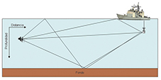
In the early 1970s, CS Miller and CE Bohman used frequency hopping to reduce the effects of multipath propagation, also employing phase modulation combined with frequency modulation [5]. Of all the effects present, multipath propagation was identified as the main difficulty in establishing communication. This effect is more noticeable in transmissions along the distance axis, since more reflections occur than in a transmission along the depth axis. Figure 1 represents a situation where propagation occurs along the distance axis, and where different paths appear that the signal can follow to the receiver (direct path, a reflection off the bottom, etc.), thus forming the multipath.
Transmission speeds achieved during the 1980s were around one kilobit per second in experiments using frequency modulation or phase modulation, such as those described in [6] or [7].
In the 1990s, the use of phase modulation began to become more widespread, replacing frequency modulation. In 1992, using this modulation, speeds of 16 kbps were achieved in a transmission along the depth axis [8]. In 1994, R. Galvin and RFW Coates developed a system that achieved speeds of 10 kbps for transmission along the distance axis, where the transmitter and receiver were separated by 2 km [9]; when the receiver was placed 900 m from the transmitter, the transmission speed was 20 kbps. And a couple of years later, in 1996, the Woods Hole Oceanographic Institution developed a system that reached speeds of 40 kbps for a distance of 2 km [10].
From this point onward, the various contributions focus less on increasing speed and more on employing different configurations. To name a few examples, in 1999, a system developed by E.M. Sozer et al. appeared, based on the Direct Sequence Spread Spectrum (DSSS) technique [11]. In 2004, D. Kilfoyle used spatial modulation and a multi-user receiver that takes advantage of the spatial variability of multipath propagation, achieving a two- to three-fold increase in channel capacity [12]. Increasingly, studies began to appear on implementing underwater sensor networks, such as the one published by Akyildiz et al. in 2005 [13], and other modulation possibilities emerged, such as Orthogonal Frequency Division Multiplexing (OFDM) [14]. In 2007, S. Roy et al. They propose space-time coding along with iterative equalization, obtaining speeds of 48 kbps [15].
 Fundamental Parameters of Underwater Acoustic Propagation:
The speed of sound and transmission losses are the two fundamental parameters regarding the propagation of an acoustic wave in an underwater medium. The variation of the speed of sound with depth determines what is known as the "speed of sound profile," which, depending on its shape, will favor the propagation of the acoustic wave in a particular way. Transmission losses are due to the various factors that attenuate the acoustic wave as it travels through the underwater medium.
Speed of sound
Strictly speaking, the speed of sound is obtained from the linear wave equation [1], and its value is that which appears in equation (1):
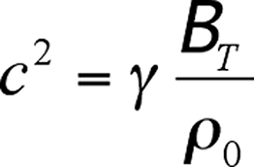 Where c is the speed of sound in m·s⁻¹, g is the adiabatic index, BT is the isothermal bulk modulus, and ρ₀ is the equilibrium density. These three quantities are functions of the water's temperature and pressure.
Obtaining an expression that clearly reflects these variations is complex, so it is common to express the speed of sound using semi-empirical expressions, which then depend on the measurements taken, resulting in a large number of equations. For example, one equation for distilled water is expressed in equation (2) [1]:

 Where c is the speed of sound in m·s⁻¹, t = T/100, where T is the temperature in degrees Celsius, and is the gauge pressure expressed in bars, where a value of 0 bar indicates an equilibrium pressure of 1.01325 bar (1 atm). This equation is valid for temperatures between 0°C and 100°C, and gauge pressures between 0 and 200 bar.
The most commonly used underwater medium for the propagation of acoustic waves is the ocean (or the various seas), and therefore, the terms seabed or ocean floor, as well as the sea surface, will be used by default, although the results can be extrapolated to other underwater environments. Seawater differs from distilled water with respect to the variables that influence the speed of sound, introducing another factor: salinity. Over the past few decades, several equations have emerged to express the speed of sound in marine environments, the most important being the Del Grosso and Chen and Millero equations. The latter was recognized by UNESCO as the standard algorithm for calculating the speed of sound in underwater environments [16].
The Del Grosso equation originally dates from 1974 and is expressed, in its subsequently corrected form, as equation (3). The DCi coefficients, in turn, encompass other coefficients (a total of 18) that can be a function of temperature (T), pressure (P), and salinity (S) [16]:
 This equation is valid for temperatures between 0ºC and 30ºC, salinities between 30‰ and 40‰, and pressures between 0 kg·cm2 and 100 kg·cm2.The
Chen and Millero equation, for its part, dates from 1977, and in its subsequently corrected form is expressed according to equation (4), where, as in the previous case, the coefficients that appear encompass others (a total of 42), which may depend on the temperature (T), pressure (P) and salinity (S) [16]:

 This equation is valid for temperatures between 0°C and 40°C, salinities between 0‰ and 40‰, and pressures between 0 and 1000 bar.
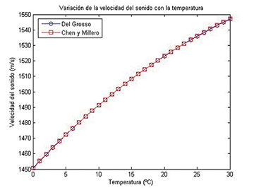
There is no appreciable difference between the results obtained by both equations within the overlapping ranges of validity. For example, one can study how the velocities obtained by both expressions vary with temperature. This result is shown in Figure 2, where it can be seen that the obtained value is practically identical. An analogous result is obtained when considering variations with pressure or salinity.
Once a value for the speed of sound is obtained as a function of temperature, pressure, and salinity, one can study how this speed varies with depth to obtain the sound speed profile. To do this, it is necessary to know how temperature, salinity, and pressure vary with depth.
 In general, salinity varies with depth by negligible, except in specific regions such as polar zones or estuaries. The speed of sound varies by 1 m/s for every part per thousand change in salinity, and salinity typically varies no more than 3‰ in a given region, and 10‰ between different oceans and areas of the world. Furthermore, the speed of sound varies by 5 m/s for every degree Celsius, and by 1.6 × 10⁻⁶ m/s for every Pascal, where both temperature and pressure depend on depth [3]. The variation of the speed of sound with pressure may seem negligible, but pressure increases at a rate of 1 atm for every 10 m of depth. At 1 km, the pressure would be approximately 100 atm, or 10,132,500 Pa, so the speed of sound varies by approximately 16 m/s in the first kilometer [1]; this effect is noticeable in the oceans, where the depth can reach several kilometers.
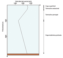
Taking all these effects into account, the sound speed profile is obtained, which for mid-latitudes has the typical shape shown in Figure 3. At great depths, the temperature remains practically constant, so since salinity hardly varies with depth, changes in the speed of sound are due to the variation in pressure with depth. Pressure decreases as the surface gets closer, so the speed of sound also decreases. In Figure 3, this behavior occurs down to a depth of around one kilometer, where a minimum in the speed of sound occurs. The region from the ocean floor to this minimum is called the deep isothermal layer.
At depths less than this, the effect of temperature begins to be noticeable, increasing as one approaches the sea surface. This effect is more significant than the variation of pressure with depth. This zone, extending from 1000 m to a depth of approximately 200 m, is called the main thermocline, and the effect of the seasons is negligible within it. Between 200 m and 100 m, there is a region where seasonal effects are indeed appreciable, so the shape of the profile in this region varies depending on the season. This region is called the seasonal thermocline. Below 100 m, the surface becomes exposed to atmospheric changes, such as wind, abrupt temperature changes, and the movement of water masses. This movement of water masses produces mixing that allows this region to be considered isothermal, despite any abrupt temperature changes it may experience. For this reason, it is called the surface layer or mixed layer.
The profile described here is valid for mid-latitudes, but it generally varies with latitude and local conditions. For example, in a polar region, the temperature does not increase with depth, so the deep isothermal layer extends to the surface. In other areas, the depth of the minimum speed of sound may differ from one kilometer.
Once the shape of the speed of sound profile is known, it is possible to determine how the acoustic signal will propagate through the underwater medium. Due to Huygens' principle and given the shape of the speed of sound profile, zones are formed where waves arising from wavefronts propagate at different speeds depending on the depth of those wavefronts. The net effect is the bending of the acoustic wave towards the region where the speed of sound is lower. The shape of the sound speed profile and this effect of the curvature of acoustic waves towards areas where this speed is lower, is key to the appearance of different types of propagation, as will be seen later.
Transmission Losses.
In the propagation of an acoustic signal through the underwater medium, it will suffer various losses due to three main contributions: geometric divergence, absorption by the medium, and reflections from surfaces. These losses are encompassed by a parameter called transmission loss, TL (transmission loss).
Geometric divergence occurs as a consequence of the propagation of the acoustic wave. The natural shape of propagation of an acoustic wave is spherical, and therefore the energy carried by the signal is distributed as the distance increases. However, when the relationship between the distance at which the wave propagates and the depth of the seabed is such that the wave is confined between the surface of the sea and the seabed, the propagation is considered cylindrical.
Transmission losses are typically calculated from the acoustic intensity, although it is more convenient to use an expression as a function of distance. For a given distance r, the transmission loss due to geometric divergence, if it is spherical, is twice that of cylindrical divergence. Specifically, for spherical divergence the transmission losses, in dB, are given by (5), and for cylindrical divergence, by (6) [1]:
 During the propagation of an acoustic signal, some of its energy is transferred to the medium as heat; this process is known as absorption by the medium and consists of two main contributions: the viscosity of the water and relaxation processes. In freshwater, only the first contribution appears, while the second appears in saltwater due to the ionic relaxation processes of magnesium sulfate and boric acid.
These contributions are captured in the parameter called the absorption coefficient, which is expressed semi-empirically, with various formulas developed over the last few decades. One of the most widely used expressions is Thorp's (7), which dates from the late 1960s and is valid up to frequencies of a few kilohertz [17]:

 Where a has units of dB·km-1 and f is the signal frequency in kHz. The last term is a correction that takes into account absorption at very low frequencies, this equation being valid for temperatures of 4ºC and a depth of 900 m, which is where the measurements were taken [2].
Another more modern expression, from the early 1980s, is that provided by Francois and Garrison, valid for frequencies between 100 Hz and 1 MHz, and which is expressed according to equation (8) [18]:
 Where a has units of dB·km⁻¹ and f is the signal frequency in kHz. The first term comes from the contribution of boric acid, the second from the contribution of magnesium sulfate, and the third from the viscosity of water. f₁ and f₂ are the relaxation frequencies of boric acid and magnesium sulfate, respectively, in kHz, and the coefficients Ai and Pi can depend on pH, salinity, depth, temperature, and the speed of sound.
Using the Francois-Garrison equation, the graph shown in Figure 4 was obtained, representing the variation of the absorption coefficient with frequency, for the range between 100 Hz and 1 MHz. This result was obtained for a pH of 8, salinity of 35‰, temperature of 5°C, and a depth of 0 m.
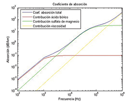 An important conclusion can be drawn from Figure 4: for transmissions over long distances, on the order of several kilometers, frequencies on the order of tens of kHz should be used, since otherwise the absorption will be too great; for transmissions over short distances, less than 1 km, frequencies on the order of hundreds of kHz could be used.
 The final contribution to transmission losses is due to signal reflections off the sea surface or seabed. In the case of the sea surface, if it is perfectly smooth, the reflection can be considered specular, and very little energy is lost in the process. If the surface is not smooth, part of the signal will be reflected in directions other than it would be in the case of specular reflection, resulting in energy loss. The Rayleigh parameter, given in equation (9), is commonly used to characterize the regularity of the sea surface [19]:
where k is the wave number, q is the angle of incidence on the sea surface, and 2a is the RMS value of the wave height, from its highest to its lowest point, considering the highest third of the waves. Through various experiments, it has been determined that for frequencies below 1 kHz, transmission losses are 1 dB/reflection, while for frequencies above 25 kHz, these losses are around 3 dB/reflection [19]. This increase in losses is due to the fact that as frequency increases, wavelength decreases. Therefore, smaller surface irregularities, which would go unnoticed at longer wavelengths, will affect the reflection.
The study of the seabed is, in principle, analogous, although more complex due to the irregularity of the seabed's terrain and composition. Several models attempt to reproduce the behavior of acoustic signal reflections off the seabed, ranging from the ideal Rayleigh model to others such as the Sommerfeld model or geoacoustic models. In addition to signal reflection off the seabed, the layer of sediment above it must also be considered, as it contributes to signal attenuation.
Taking into account all the contributions discussed, transmission losses can be expressed according to equation (10) for spherical propagation, or equation (11) for cylindrical propagation:
Where the distance r, which is where the losses are to be measured (generally at the receiver), is expressed in meters, and the contribution of reflections has been left generic, as it depends on too many conditions and models to give an explicit expression.
[References at the end of Part Three]
Author:
Joaquín Aparicio, Enrique García; Ana Jiménez; Fernando Álvarez†; Jesús Ureña
Department of Electronics, University of Alcalá
†Department of Electrical, Electronic and Automatic Engineering, University of Extremadura