This article will not delve into the mathematical models, although the results provided by the ray tracing model, the most versatile and widely used, will be briefly discussed below. The ray tracing model is based on the premise that wave energy can be concentrated along defined paths, allowing us to think of them as rays rather than waves. This assumption holds true as long as the wave amplitude and the speed of sound do not vary significantly over a wavelength, a condition that is best met at high frequencies due to their smaller wavelengths. The ray tracing model calculates the equations governing the rays, as well as the pressure field they generate, from which transmission losses and the propagation time of these rays can be determined.
Propagation in Shallow Water:
When the depth of the seabed is such that multiple signal reflections occur between the sea surface and the bottom, propagation is considered to be taking place in a shallow water environment. Figure 1 can serve as a graphic example of this type of transmission.
In shallow water propagation, there is a significant interaction between the acoustic signal and the seabed. This interaction is quite complex, as it is necessary to consider the type of seabed, the sediments, their distribution, and any variations in depth, among other factors. All these difficulties make the use of mathematical models such as ray tracing risky. Semi-empirical models then emerge, among which the Colossus model [20] stands out.
This model was derived from a series of measurements taken between 100 Hz and 10 kHz. It takes into account wave height (depending on sea state), seabed type, water column depth, frequency, and the sound speed profile. This profile is considered to consist of two constant segments: from the sea surface to a certain depth L, in meters, the speed of sound increases linearly with depth, while for depths greater than L, the speed decreases with depth until reaching the bottom.
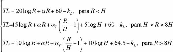
If the skip or transmission distance, H, is defined as the maximum distance at which a ray makes contact with the surface or the bottom as given in equation (12), where D is the depth of the water column in meters, the transmission losses are obtained according to the equations given in (13) [20]:

(12)
(13)
Where R is the distance in km, a is the absorption coefficient in dB·km-1, kL is a parameter called the near-field anomaly, which measures the gain due to reflections between the bottom and the surface, in dB, and aT is the so-called effective attenuation coefficient, which takes into account the losses due to energy coupling between the surface and the bottom, expressed in dB/reflection. The values of these last two coefficients are tabulated for different types of bottom and sea state, for example in [2].
The surface channel
: The region of the water column near the surface is where the most significant temperature variations occur. However, the movement of water masses caused by waves mixes the water in this region, so it can be considered isothermal. If the salinity is constant, the speed of sound varies only with depth, resulting in a positive gradient of the speed of sound with depth down to a certain depth, where the thermocline appears.
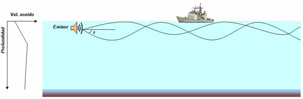
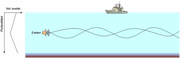
Since acoustic waves bend towards areas of lower sound speed, if a transmitter is placed in this region near the surface, called a surface channel, the acoustic waves will be trapped within it if the emission angle is sufficiently small and the wavelength is no greater than the width of the channel. Thus, the acoustic signal propagates by bouncing off the sea surface and curving to bounce back off the surface, without touching the bottom, as shown in Figure 5.
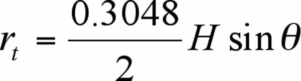
It should be noted that the signal propagates spherically at first, but beyond a certain distance rt, called the transition distance, the propagation can be considered cylindrical, as the energy is confined. In this case, the transmission losses can be expressed according to equation (14), where the transition distance is given by equation (15) [2]:
 (14)
(14)
(15)
Where r is the distance in meters, a is the absorption coefficient in dB·km-1 and aL is the so-called leakage coefficient, also in dB·km-1. This leakage coefficient takes into account the energy that escapes from the channel due to signal scattering on the surface and transverse diffusion, which originates from the discontinuity of the sound speed profile at the base of the channel; H is the depth of the channel in meters, and q is the angle of the most inclined trapped ray within the channel, as shown in Figure 5.
The Deep Acoustic Channel.
Figure 3 shows a typical profile for mid-latitudes. In this profile, at a depth of approximately 1 km, a minimum in the speed of sound appears. This minimum marks the so-called axis of the acoustic channel, and an acoustic signal emitted near this depth will curve towards it. Therefore, if the emission angle is sufficiently small, the signal propagates without bouncing off the surface or the seabed. This forms a propagation channel, called the deep acoustic channel, represented in Figure 6.
In this case, transmission losses are due to the geometric divergence of the signal and absorption by the water. Initially, the geometric divergence will be spherical, until it reaches the transition distance rt, beyond which it can be considered cylindrical. There is no further contribution due to reflections off the seabed or surface. Transmission losses can be expressed in the form given in (16), provided that the distance r is such that the divergence is either cylindrical [1]:
 (16)
(16)
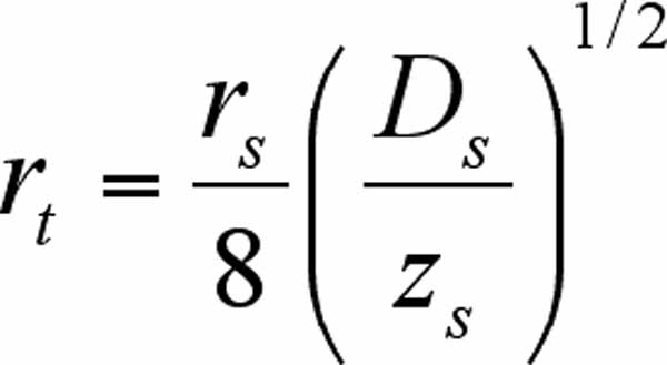
Where r is the distance in meters where the transmission losses are to be calculated, and is the absorption coefficient in dB·km-1. The transition distance can be calculated according to equation (17) [1]:
(17)
Where Ds is the depth at which the minimum speed of sound is found in the surface channel, zs is the depth of the emitter measured from the base of the surface channel, which marks the beginning of the deep acoustic channel, and rs is the skip distance. This skip distance depends on the distances between the acoustic axis and the limits of the deep acoustic channel, the value of the speed of sound at the base of the surface channel, and the difference between this value and the minimum, obtained at the axis of the acoustic channel.
Other Propagation Modes and Additional Comments
We have discussed so far the three most relevant channels in acoustic propagation in terms of the importance of the sound velocity profile, but other propagation modes exist. In addition to the direct path, i.e., direct transmission between transmitter and receiver, which occurs for very short distances, we must highlight convergence zones, the reliable acoustic channel, and arctic channels.
 Convergence zones form due to the accumulation of rays in a specific area near the surface, but without touching the seabed or the surface itself, resulting in signal reinforcement. In these zones, transmission losses are lower due to the appearance of a term called convergence gain.
A reliable acoustic channel occurs when there is a transmitter at a great depth, below the acoustic axis, and a receiver near the surface. When the signal is transmitted, the deep isothermal layer causes the rays to curve towards the surface, where they reach the transmitter without touching either the seabed or the surface. Since it does not interact with either, it is considered reliable.
In Arctic channels, there may be an ice layer on the sea surface, which introduces an additional source of noise due to the breakup and falling of ice fragments into the water, and greater uncertainty in ray reflection due to the irregularity of this ice layer, as well as scattering processes. The temperature conditions in these regions create a sound speed profile where the speed increases linearly with depth, meaning the acoustic axis can be considered to be at the surface. All emitted rays will eventually curve towards the surface, bounce off it, and interact with the ice layer, which acts as a low-pass filter due to scattering.
In general, the models studied can provide a good approximation of the transmission loss values that would be obtained for a given case. However, there are additional factors that can influence the result and are not present, such as turbulence, eddies, internal currents, or ambient noise. All these factors can alter the results obtained, as will be discussed in the second part of this work.
[References at the end of the third part]
Author:
Joaquín Aparicio, Enrique García; Ana Jiménez; Fernando Álvarez†; Jesús Ureña
Department of Electronics, University of Alcalá
†Department of Electrical, Electronic and Automatic Engineering, University of Extremadura