However, considering only these effects would constitute an ideal case within practical applications. Numerous additional mechanisms can appear when acoustic propagation occurs in underwater environments, some of which will cause signal fluctuations in both amplitude and phase. By default, we will refer to marine environments, but these effects can generally occur in other underwater environments as well.
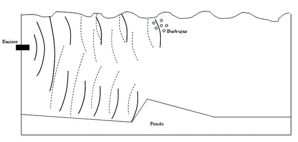
One mechanism that will always appear is reverberation. Reverberation is the energy dispersed in other directions as a result of the interaction of acoustic waves with the medium, such as reflections off surfaces or the encounter of waves with suspended particles in water. Figure 7 shows an example of different reverberation processes, where the reflected signal that causes reverberation appears as a dashed line.
 Two types of reverberation can be considered: volumetric and surface. Volumetric reverberation occurs within the volume of water where propagation takes place and is primarily due to suspended particles and the presence of marine life. The contribution of the deep scattering layer, of biological origin, to volumetric reverberation is particularly noteworthy, as it provides a higher level of scattering than the rest [2]. Due to this biological origin, the depth of the deep scattering layer varies throughout the day, depending on the movement of animals, and its response to different frequencies of the acoustic signal, which depends on the size of the animals, indicating that it is composed of several sublayers.
Surface reverberation results from scattering caused by the interaction of acoustic waves with nearby surfaces and particles, such as sediment or layers of bubbles introduced by waves or passing ships. At the sea surface, the level of scattering depends on the frequency, the angle of incidence, and the irregularity of the surface, which in turn depends on the surface wind speed [2]. If there is also an ice layer on the surface, the reverberation will be greater. At the bottom, the level of scattering also depends on the material: rocky bottoms produce more reverberation than sandy bottoms. The contribution of the seabed to reverberation is the most complex to predict, since the interaction of acoustic waves with the seabed is the most difficult to determine.
Furthermore, the gas bubbles present in the water become part of the compression and rarefaction processes of the wave, where the magnitude of this response to the acoustic signal will depend on the frequency and size of the bubbles. In this process, the acoustic waves lose energy to the bubbles, which radiate it in all directions, causing reverberation, which will be at its maximum when the bubbles resonate [2].
In addition to this effect, and although it is not reverberation, it is worth mentioning that gas bubbles cause variations in the speed of sound as it passes through a region where a layer of bubbles is present. If the size of the bubbles is smaller than the resonant size for the signal frequency, the bubble is compressed during the compression phase of the acoustic wave, thus reducing the bulk modulus and consequently the speed of sound; if the size is larger, the bubble expands during the compression phase, increasing the bulk modulus and consequently the speed of sound [3]. These variations in the speed of sound will affect the shape of the airfoil, with the resulting consequences.
 In general, if a sinusoidal pulse is emitted, the reverberation signal will appear as an irregular tone that decays over time, although intensity peaks may occur at certain moments. This tone will undergo frequency shift and spectral broadening due to the movement of suspended particles, marine life, the possibility that the reverberation received from different directions may have undergone different Doppler shifts, and so on. The reverberation will be greater as the transmitted power increases and the acoustic signal is emitted over a wider range of angles.
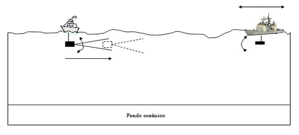
The Doppler effect is another mechanism to consider. Given the nature of the underwater environment, the transmitter or receiver (or both) may be in motion when measurements are taken, such as on a boat (Figure 8). In this case, the Doppler effect occurs, consisting of a frequency shift. If the signal can travel along different paths (multipath), different Doppler shifts appear, resulting in a broadening of the spectrum at the receiver.
 Furthermore, even if the instruments were perfectly still, Doppler broadening can still occur due to the movement of water masses during signal transmission, such as that caused by waves, which alter the reflecting surface. Another contribution can come from internal currents, causing the displacement of water masses, which will affect acoustic propagation.
To avoid the consequences of this broadening, the signal duration must comply with the relationship given in expression (18) [7]:
1
__ >> B (18)
T
Where T is the signal duration and B is the Doppler broadening. This Doppler broadening increases with frequency, so it is especially important at short distances (one kilometer or less), where several tens of kHz can be used [4].
The Doppler broadening is of interest along with the multipath delay, which appears due to surface reflections and the refraction of the rays towards the minimum speed of sound; therefore, the arrangement of the transmitter and receiver is critical. The multipath delay is the time between the arrival of the first signal and the arrival of the signal from the longest path.
Propagation along the distance axis can cause significant temporal broadening due to multipath propagation, resulting in the effect known as intersymbol interference (ISI). For example, at a transmission rate of 10 ksps (kilosymbols per second) over a shallow water channel that can extend from 1 to 10 km, a multipath delay of 10 ms occurs, causing ISI to spread over 100 symbols [4]. To avoid the effects of these multiple multipath arrivals at the receiver, the relationship given in equation (19) [7] must be satisfied:
1
__ >> tL (19)
W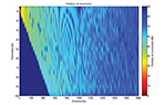 Where W is the bandwidth and tL is the multipath delay. The goal in all systems is for the product B·tL to be less than one; otherwise, the system is said to be over-spread and the channel cannot be used correctly unless the acoustic signal is pre-processed.
In addition to these effects, it is important to consider that the underwater environment is dynamic; that is, there are various processes that cause changes in the environment. These processes are usually classified according to their spatial extent as large-scale phenomena (more than 100 km), mesoscale phenomena (between 100 m and 100 km), and small-scale phenomena (less than 100 m) [19].
Large-scale phenomena include wind-driven circulation in the first few hundred meters of depth and thermohaline circulation, caused by density changes resulting from variations in water temperature and salinity.
Mesoscale phenomena include ocean fronts, eddies, and internal waves. Ocean fronts are transition zones that separate water masses with different characteristics, especially temperature and salinity. Eddies consist of water masses that flow in a circular pattern, closing upon themselves, and can therefore be considered a special case of an ocean front, as they exhibit distinct characteristics from their surroundings. Internal waves, on the other hand, are waves that propagate along the interfaces between layers of fluids of different densities, or within the same fluid that exhibits a density gradient.
Finally, among the small-scale phenomena, the thermohaline ladder stands out. It generally appears in the main thermocline and consists of zones several meters deep where temperature and salinity are uniform, separated by other zones where there is a noticeable gradient in these values. This effect occurs more frequently in areas where fresh and salt water mix.
Another mechanism to consider is the dispersion of the speed of sound (to be distinguished from scattering). Dispersion consists of the propagation at different speeds of the signal's components of different frequencies. Because it is generally not present, the semi-empirical formulas found in the literature do not take this dependence into account; however, it can appear under certain circumstances, such as passing through a layer of bubbles [21] or depending on the shape of the channel (geometric dispersion) [22]. Dispersion effects can be very significant if the acoustic signal is encoded, since the signal may arrive unrecognizable at the receiver.
The last mechanism to consider is ambient noise, that is, any signal that continues to be received even after all known noise sources have been eliminated. This ambient noise is usually heard as a low-frequency hum, generally on the order of hertz.
In the open ocean, where deep-water propagation can be considered, there are several possible sources of ambient noise: waves, tides, and turbulence, which cause pressure changes recorded by hydrophones; the breaking of waves on the sea surface and of bubbles in the water; seismic activity; the presence of ships; and the so-called thermal noise of molecules. Almost all of these contributions are low-frequency, generally below 100–500 Hz, except for the breaking of waves and bubbles, which can reach 30 kHz, and thermal noise, which can reach 100 kHz [2].
In shallow waters, the potential sources of ambient noise are also known, but their variability, both spatially and temporally, is greater. These sources include fishing and industrial noise, wind, and biological noise from marine life, such as crustaceans. Generally, ambient noise in shallow waters affects lower frequencies more, as in the previous case.
There are two further contributions. One is common to both deep and shallow waters and consists of the noise caused by raindrops hitting the sea surface. This noise can reach frequencies of 10 kHz [2]. The other contribution is specific to polar regions, where fishing and wind have a lesser impact due to the ice cover, but the breaking up of this ice is a significant source of noise that can reach frequencies of up to 1 kHz [19].
Simulations.
Several simulations performed using the ray tracing method, the most widely used in the literature, are shown below. Three fundamental cases are distinguished: shallow water channel, surface channel, and deep acoustic channel. In all cases, a water column with a density of 1024 kg·m⁻³ is considered, resting on a fine sand bottom with a density of 1941 kg·m⁻³. The presence of transverse waves on the bottom, which is perfectly smooth, as is the sea surface, is not considered. In all transmission loss calculations, the phase of the different rays has been considered (coherent calculation), since perfectly smooth surfaces have been assumed, and therefore there is no uncertainty in the interaction of the signal with these surfaces.
Simulation of a Shallow Water Environment:
The acoustic propagation in a shallow water environment, characterized by multiple reflections between the bottom and the surface, is shown first. In this particular case, the bottom is located at a depth of 100 m, and a network of receivers is assumed, positioned every 5 m at a depth, 2 km away from the emitter, which is located at a depth of 10 m.
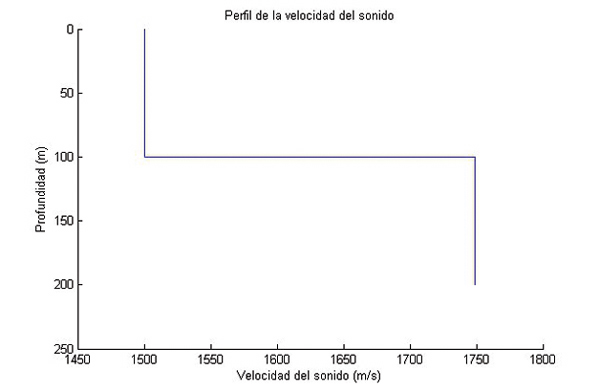
The sound speed profile is given by Figure 9, which shows a constant speed in water of 1500 m/s and a constant speed in fine sand of 1749 m/s.
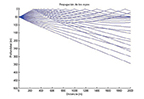
The rays are emitted at angles of ±10º, at a frequency of 30 kHz. Figure 10 shows the path these rays follow to the receiver, where 21 rays have been chosen for visual clarity. This figure shows how some rays reach the receiver network without bouncing, while others bounce off the background or surface, or bounce off both multiple times.
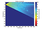
Figure 11 shows the transmission losses as a function of distance and depth. To calculate these losses, the algorithm was allowed to choose the number of rays it deemed appropriate (much greater than 21 rays). This figure shows how there are areas where the signal interferes destructively, depending on the phases of the converging signals in that area, resulting in zones where transmission losses decrease considerably at distances close to the emitter.
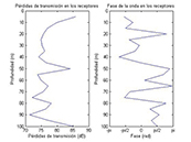
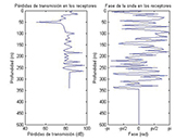
Figure 12 shows the variation of transmission losses and phase with respect to depth, for a distance of 2 km, where the receivers would be located. The values obtained for transmission losses coincide with what is expected for a geometric divergence at a distance of 2 km and the contribution of absorption, which for a frequency of 30 kHz is approximately 8 dB·km⁻¹. The phase also undergoes several fluctuations due to interaction with the sea surface and interference between different rays.
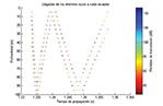
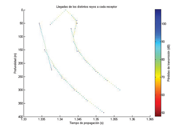
Figure 13 represents the different arrivals of rays at the receivers, that is, the multipath. For example, for the receiver located at 5 m, a first ray is detected for a propagation time of approximately 1.334 s (time consistent with the distance and speed of sound considered), then it detects five rays very close together around 1.34 s, and finally it detects another ray for a propagation time of approximately 1.357 s.
Surface Channel Simulation.
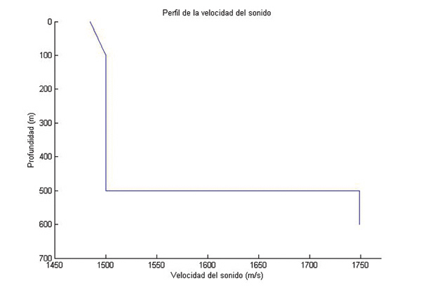
The simulation of acoustic propagation in a surface channel is now presented. The sound speed profile is shown in Figure 14, where the speed at the surface is 1485 m/s and increases to a depth of 100 m. From that point, its value is constant at 1500 m/s. The receiver network is located 2 km from the emitter, which is at a depth of 50 m, assuming one receiver every 5 m. The emission frequency is 20 kHz, with the rays emerging at angles of ±10°, and the depth to the bottom is 500 m.
Figure 15 shows the paths followed by the rays in this channel, where, as in the previous case, 21 rays were chosen for the same reason. This figure illustrates the curvature of the rays towards the surface, where the speed of sound is at its minimum. In this case, there is no interaction with the seabed at the distance of the receivers; there are only reflections off the sea surface.
Transmission losses as a function of distance and depth are shown in Figure 16. This figure shows, as in the case of shallow water, an interference pattern formed by the interaction of rays with different phases. An area now appears at the distance of the receivers and at a depth of approximately 50 m, where losses are considerably lower than in the surrounding area. This is due to the concentration of rays in this area, as can also be seen in Figure 15.
In Figure 17, which shows the variation of transmission losses and phase with depth at the receivers, this minimum in transmission losses is also shown, highlighting the clear difference in loss values at this depth. Figure 18 represents the multipath obtained for this case, which, in general, shows fewer detections for each receiver than in shallow water, except for the receiver located at a depth of 50 m. This is because there are fewer reflections between surfaces, and therefore the multipath will be shorter.
Deep Acoustic Channel Simulation
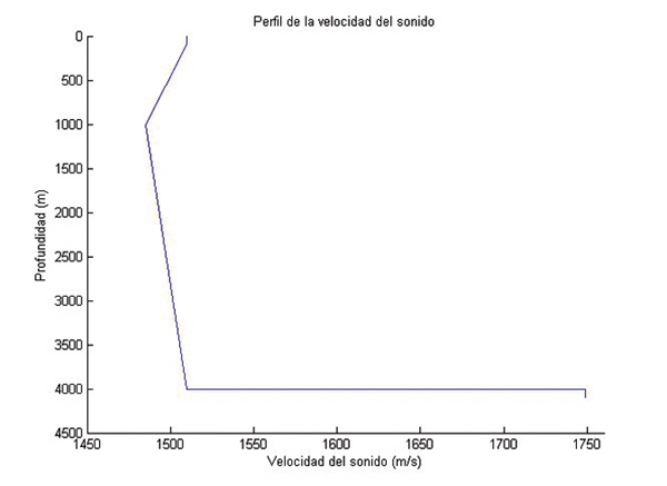
The last simulation presented is that of the deep acoustic channel. Figure 19 shows the profile considered for this case, where the velocity has a constant value of 1510 m/s from the surface to the first 100 m, then decreases to 1485 m/s at the acoustic axis, located at 1 km; it then increases linearly until reaching 1510 m/s again at the bottom, at a depth of 4 km. The receivers are located 50 km away, assuming one every 5 m, as in the previous cases; the transmitter is on the acoustic axis. In this case, a frequency of 500 Hz was used to simulate a practical scenario as closely as possible, since at 30 kHz the losses at the receivers would be around 500 dB, mainly due to absorption, making it an unfeasible frequency in reality for transmission at this distance. The rays are emitted within ±10º.
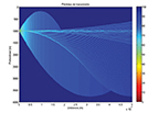
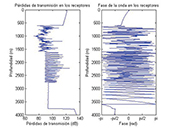
Figure 20 shows the transmission losses obtained for distance and depth. It can be seen that transmission losses in the region near the acoustic axis are lower than in other areas due to the refraction of the rays towards this zone, causing their accumulation. Figure 21 represents the variation of losses and phase with respect to depth at the receivers. This graph also shows the minimum loss obtained at the depth of the acoustic axis.
Conclusions
This article has presented a review of the fundamentals of acoustic propagation in underwater environments, highlighting the importance of understanding the sound speed profile for the subsequent propagation of a signal through various channels. The most important theoretical equations for the speed of sound, absorption, and losses for different channels have been examined, and various effects that can affect underwater acoustic propagation have been presented qualitatively. Additionally, several simulations performed for the three most significant channels have been shown.
Acknowledgments
This work was made possible thanks to the support of GCM Communications Technology. The simulations were performed using the Acoustic Toolbox for Matlab, available on the website of the Centre for Marine Science and Technology (Curtin University of Technology, Australia) [23].
Authors:
Joaquín Aparicio, Enrique García; Ana Jiménez; Fernando Álvarez†; Jesús Ureña
Department of Electronics, University of Alcalá
†Department of Electrical, Electronic and Automatic Engineering, University of Extremadura
Bibliography
[1] Lawrence E. Kinsler, Austin R. Frey, Alan B. Coppens and James V. Sanders,
“Fundamentals of Acoustics”, Ed. John Wiley & Sons, 4th Edition, 2000.
[2] Robert J. Urick, “Principles of Underwater Sound”, Ed. Peninsula Publishing,
3rd Edition, 1983.
[3] TG Leighton, chapter “Fundamentals of Underwater Acoustics”, pp. 373-443,
in Fundamentals of Noise and Vibrations, Frank Fahy and John Walker, Ed.
Taylor and Francis, 1st Edition, 1998.
[4] Milica Stojanovic, “Acoustic (Underwater) Communications”, in Wiley
Encyclopedia of Telecommunications, John G. Proakis, Ed. John Wiley &
Sons, 1st Edition, 2003.
[5] Chauncey S. Miller and Carl E. Bohman, “An Experiment in High Rate Underwater
Telemetry”, in OCEAN 84, Vol. 34-48, 1972.
[6] Azizul H. Quazi and William L. Konrad, “Underwater Acoustic Communication”, in
IEEE Communications Magazine, Vol. 20, No. 2, pp. 24-30, 1982.
[7] Arthur B. Baggeroer, “Acoustic Telemetry – An Overview”, in IEEE Journal of
Oceanic Engineering, Vol. 9, No. 4, pp. 229-235, 1984.
[8] M. Suzuki, T. Sasaki and T. Tsuchiya, “Digital Acoustic Image Transmission
System for Deep-Sea Research Submersible,” in OCEANS'92 Proceedings,
Vol. 567-570, 1992.
[9] R. Galvin and RFW Coates, “Analysis of the Performance of an Underwater
Acoustic Communications System and Comparison with a Stochastic Model,”
in OCEANS'94 Proceedings, Vol. 478-482, 1994.
[10] Milica Stojanovic, “Recent Advances in High-Speed Underwater Acoustic
Communications,” in IEEE Journal of Oceanic Engineering, Vol
. 125-136, 1996.
[11] EM Sozer, JG Proakis, M. Stojanovic, JA Rice, A. Benson and M. Hatch,
“Direct Sequence Spread Spectrum Based Modem for Underwater Acoustic
Communication and Channel Measurements,” in Proceedings of MTS/IEEE
OCEANS'99, pp. 228-233, 1999.
[12] Daniel Kilfoyle, “Spatial Modulation in the Underwater Acoustic Channel.”
Edited by Ft. Belvoir Defense Technical Information Center. Page
managed by Massachusetts Institute of Technology, available at:
http://www.ll.mit.edu/asap/asap_04/DAY2/36_PA_KILFOYLE.PDF
[13] Ian F. Akyildiz, Dario Pompili and Tommaso Melodia, “Underwater Acoustic
Sensor Networks: Research Challenges”, in Ad Hoc Networks, Vol
. 257-279, 2005.
[14] Milica Stojanovic, “OFDM for Underwater Acoustic Communications: Adaptive
Synchronization and Sparse Channel Estimation,” in IEEE International
Conference on Acoustics, Speech and Signal Processing (ICASSP) 2008,
pp. 5288-5291, 2008.
[15] Subhadeep Roy, Tolga M. Duman, Vincent McDonald and John G. Proakis, “High-
Rate Communication for Underwater Acoustic Channels Using Multiple
Transmitters and Space-Time Coding: Receiver Structures and Experimental
Results,” in IEEE Journal of Oceanic Engineering, Vol. 663-
688, 2007.
[16] “Technical Guides: Speed of Sound in Sea-Water”, page managed by
Communication Technology. Available at:
http://www.comm-tec.com/Library/Technical_Papers/speedsw.pdf
[17] Milica Stojanovic, “On the Relationship Between Capacity and Distance in an
Underwater Acoustic Communication Channel,” in Proc. First ACM
International Workshop on Underwater Networks (WUWNeT'06) / MobiCom
2006. Available at:
http://www.mit.edu/~millitsa/resources/pdfs/wuw37-stojanovic.pdf
[18] Mari Carmen Domingo, “Overview of Channel Models for Underwater Wireless
Communication Networks”, in Physical Communication, Vol
. 163-182, 2008.
[19] Paul C. Etter, “Underwater Acoustic Modeling and Simulation”, Ed. Taylor and
Francis, 3rd Edition, 2003.
[20] M. Schulkin and JA Mercer, “Colossus Revisited: A Review and Extension of the
Marsh-Schulkin Shallow Water Transmission Loss Model”, Applied
Physics Laboratory, University of Washington, APL-UW 8508, 1985.
[21] Herman Medwin and Clarence S. Clay, “Fundamentals of Acoustical
Oceanography”, Ed. Academic Press, 1st Edition, 1998.
[22] IB Esipov, OE Popov, VA Voronin and SP Tarasov, “Dispersion of the Signal
of a Parametric Array in Shallow Water”, in Acoustical Physics, Vol
. pp. 76-80, 2009.
[23] Center for Marine Science and Technology, page managed by Curtin
University of Technology, available at: http://cmst.curtin.edu.au.