 2.0. Meltback with Variable Power
2.1. Variable Power Meltback Method Process
When a cut fiber end is heated by a very short arc discharge, in the range of 0.3 seconds to 1 second, the fiber end will not change if the arc power is too weak. If the same fiber end is heated several times using the same arc time, but gradually increasing the arc power, we can observe that at a certain power level, the corner of the fiber end will begin to round again, as shown in Figure 3.
A few key techniques are employed in the variable arc power fusion process. First, the arc heating time is very short and varies depending on the fiber diameter being measured. For 125-micron diameter fibers, the arc time can be as little as 0.3 seconds, instead of a few seconds in traditional fusion. Second, the arc power starts at a low level and is increased in small steps, just enough to prevent the fiber end from warping too quickly. Third, corner fusion can be measured in many different ways. For example, the starting point of warping at the corner can be measured, as shown in Figure 3. The change in the fiber corner radius or the variation in the corner zone can also be measured as indicators of the amount of fusion. In this article, the first definition, shown in Figure 3, step 4, is used as the fusion value.
1. Measure the center of the arc.
2. Measure the distance from the gap to the corner of the fiber.
3. Heat the ends with a low-power arc.
4. Measure the fusion at the corner of the fiber (Gap2-Gap1).
5. Increase the arc power and repeat steps 4 and 5.
6. Calculate the desired arc power from the angle of the fused corner.
2.2. Arc Power Calibration
As shown in Figure 4, the fiber end fusion defined in Figure 3, step 4, is measured for different arc power levels and plasma zone configurations. Each curve in Figure 4 represents a fusion test, consisting of 20 to 30 re-arcs of 0.3 seconds arc length, but with varying arc power. The arc power level varies from 0 bit (~10.5 mA) to 100 bit (~14.5 mA) in 25-bit increments. Between each power increment, 5 re-arcs were performed at constant power to determine the fusion rate. Five tests were performed for each plasma zone configuration, which varies from an electrode spacing of 1 mm to 3 mm, in 1 mm increments, to check for consistency. All tests are shown in the figure. 4, SMF28 was used to compare the melting rate and study the stability of the method.
It can be clearly seen in Figure 4 that when the arc power is constant, each fusion curve increases linearly, corresponding to a constant fusion rate. Each time the arc power increases, the steeper slopes of the fusion curves indicate a faster fusion rate. The fusion rate can therefore be calculated in each region of constant arc power, as indicated by the red step curve. The calculated fusion rate is represented in Figure 5(a). We also observe that the fusion rate is related to the temperature of the fiber ends. Because the fusion rate is measured in pixels with digital images, we can use pixels as the unit of measurement and thus measure the fusion rate (related to the fiber temperature) shown by the Y-axis in Figure 5 in pixels per re-arc. Furthermore, all the melting rate curves in Figure 5(a) can be approximated by parabolic curves, since the actual heat energy applied to the fiber end is proportional to the square of the arc current, which is denoted by the x-axis in Figure 5. Figure 5 also shows that a larger distance between the electrodes indicates a higher melting rate and a higher temperature at the fiber end. This means that in order to obtain the same temperature at the fiber end in different plasma zone configurations, we have to apply different actual arc powers.
 From Figure 5, a desired target curve (in red) can be mathematically fitted. This target curve can be either a curved or a straight line. We can use this target curve to regulate the nominal (not actual) arc power with the melting rate. The same target curve can be used for all different plasma zone configurations. A set of correction factors can be introduced to generate the same melting rate with the same nominal arc power settings. Figure 5(b) shows the same melting rate data as Figure 5(a), but instead shows the nominal arc power on the X-axis. The nominal arc power is used by operators to set their desired power. The goal of arc calibration is to project the actual arc power to the nominal arc power. In other words, we can use arc calibration to find the set of correction factors. This set of correction factors will then be used to create a new nominal arc power domain. Within the new domain, the same arc power setting will generate the same temperature at the fiber end (and therefore the same melting rate) regardless of the fiber diameter, electrode condition, plasma zone configuration, or ambient conditions. Calculating the correction factor is straightforward. The difference between the target curve and the measured melting rate curve can be used as the set of correction factors.
(a) Melting rate vs. actual arc power.
(b) Melting rate vs. nominal arc power.
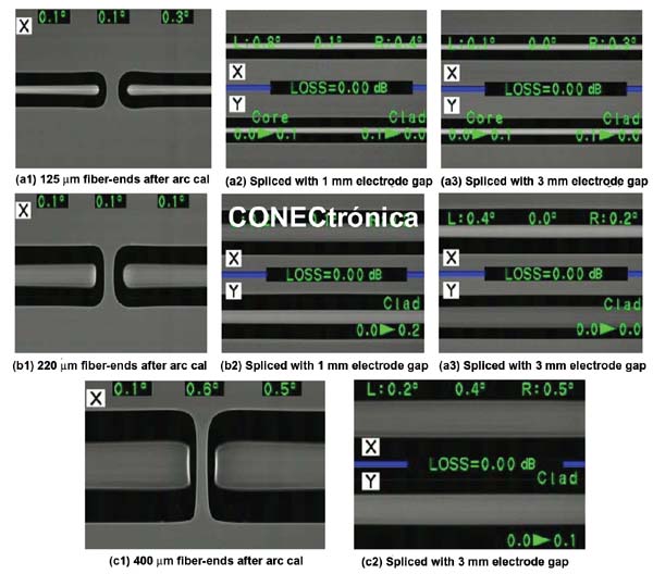
2.3. Arc calibration results
(a1) 125 µm fiber end after arc calibration.
(a2) Spliced with a 1 mm electrode gap.
(a3) Spliced with a 3 mm electrode gap.
(b1) 220 µm fiber end after arc calibration.
(b2) Spliced with a 1 mm electrode gap.
(b3) Spliced with a 3 mm electrode gap.
(c1) 400 µm fiber end after arc calibration.
(c2) Spliced with a 3 mm electrode gap.
From the examples shown in Figure 6, we can see the results of the new arc calibration method. Using the arc calibration method described above, 125, 220, and 400 micron fibers can be spliced with the same arc power setting in different plasma zones.
In other words, arc calibration operators can easily achieve the desired splicing results for different fiber types and different plasma (electrode) conditions.
For any new or unknown fiber type, engineers can easily adjust the cutting and splicing parameters using the same power setting without the tedious search for the appropriate power level.
The images of the fiber ends after arc calibration in Figure 6 also show limited core fusion and limited fiber shape distortion.
In comparison, the traditional fusion method in Figure 1(c) exhibits significantly higher levels of deformation. This new fusion method has a very limited impact on the electrode tip condition, especially for large-diameter fibers, which are prone to degraded electrode conditions when using more traditional methods.
As discussed in previous sections, both traditional fusion and offset splicing methods require multiple fiber end preparations and cuts, as cut fiber ends were no longer readily available due to the fusion or cut-and-splice process. While fiber end preparation might not be tedious for standard 125-micron telecommunications fibers, multiple fiber end preparations for larger diameter fibers could be both expensive and time-consuming. With the new method described in this article, re-cutting is unnecessary because the arc starts from very low power and gradually increases to the desired level in a continuous re-arc process.
3.0. Summary
A new arc calibration method is developed for fusing optical fibers across a wide range of glass diameters, yielding consistent and accurate results. This method heats the fiber with multiple short arcs and measures the fusion at the corner of the fiber ends.
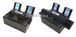
The fusion rate at the fiber corner is proportional to the fiber temperature. By varying the arc power using continuous re-arcs, an ideal fusion rate can be achieved. This ideal fusion rate represents the desired arc power for fiber testing and fusion. This method was successfully tested for fiber diameters from 60 to 1000 microns on Splice Master fusion splicers, as shown in Figure 7, with a controllable plasma zone.
The method can automatically select the correct arc power for different fiber sizes.
It allows operators to easily transfer optimized splicing parameters to multiple fusion splicers on production lines, resulting in consistent, high-quality splices.
(a) FSM 100P fusion splicer for fibers up to 500 mm.
(b) FSM 100P+ fusion splicer for fibers up to 1200 mm.
4.0. Acknowledgments
The authors wish to thank N. Kawanishi and his team in Fujikura, Japan, for their support in this work, and D. Duke and S. Althoff for their constructive comments and corrections to the article.
Author:
By Wenxin Zheng and Bryan Malinsky
References
[1] Dong, L., Mckay, H. Marcinkevicius, A., A., Fu, L., Li, J., Thomas, BK, and Fermann, ME, “Extending Effective Area of Fundamental Mode in Optical Fibers,” J. Lightwave Technol. Vol. 27, pp. 1565-1570 (2009).
[2] Even, P., Pureur, D., “High power double clad fiber lasers: a review”, Proc. SPIE – Int. Soc. Opt. Eng., 4638 pp. 1-12 (2002).
[3] Jiger, M., Verville, P., Caplette, S., Martineau, L., Brulotte DA, Gagnon, D., Villeneuve, A. “All-Fiber, Single-Stage Laser Assemblies with 91W Single-Mode, Continuous-Wave Output Power,” Quantum Electronics and Laser Science Conference (QELS), p. JWB59 (2005).
[4] Duke, D., Zheng, W., Sugawara, H., Mizushima, T., and Yoshida, K., “Plasma zone control for adaptive fusion splicing capability”, Proc. SPIE, Photonic West (2012).
[5] Zheng, W., “Automatic current selection for singe fiber splicing,” US Patent 5,909,527, Ericsson Cables, June (1999).
[6] Inoue, K., Sasaki, K., Suzuki, Y., Kawanishi, N., and Tsutsumi, Y., “Method for fusion splicing optical fiber and fusion splicer,” US Patent 6,294,760, Fujikura, Sept. (2001).
[7] Takayanagi, H., and Hatori, K., “Method for calibrate discharge energy of optical fiber splicing device,” US Patent. 7,140,786, Sumitomo, Nov. (2006).
[8] Hatori, K., “Method of determining heating amount, method of fusion splicing, and fusion splicer,” US Patent application no. 11/317899, Sumitomo, Aug. (2006).