 Among the advantages of optical networks, we can list greater range, higher transmission rates, transparency, and so on. However, these benefits come at the cost of increased complexity in monitoring and fault management. Transparent networks require managing network faults at the physical layer itself, where optical performance monitoring techniques must oversee the quality of multiple high-speed WDM channels and detect any potential degradation. Signal degradation in an optical network can be classified into three main groups: noise, distortion, and jitter. Typical noises include RIN and ASE. Signals can also suffer distortion due to chromatic dispersion, chirp, and nonlinear effects such as four-wave mixing or Raman scattering. Finally, jitter also represents a significant limitation for high speeds. In previous articles, we have analyzed in detail the measurement and characterization procedures for many of these degradations, presenting several laboratory instruments that assist in these tasks.
 However, these parameters are not usually suitable for monitoring the quality of signals in real time.
The key parameter for monitoring the performance of a digital communication system is the bit error rate (BER). This parameter ultimately determines the quality of the digital signal. However, BER measurements require photodetection of the signal in the case of an optical network. Therefore, an alternative parameter is needed, one that correlates with the bit error rate but, unlike the latter, can be monitored in the optical domain relatively easily. Fortunately, this parameter exists and is known as OSNR (optical signal-to-noise ratio). The relationship between this parameter and the bit error rate is given by the following expression (IEC 61280-2-7):
![]()
Since OSNR is a measure of average power, it cannot reveal temporary degradations in the data, nor certain bit errors. However, its correlation with BER through the above expression provides preliminary information about network performance, making it a very useful parameter for real-time monitoring of WDM channels and contributing to the generation of alarm signals that indicate possible BER degradation.
Definition and Measurement of OSNR using OSA:
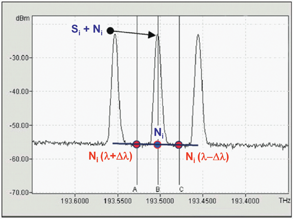
OSNR is defined as the ratio between the average signal and noise power for a given optical channel. Typically, each channel consists of virtually monochromatic modulated light (signal) over a noise power density distributed across a large bandwidth. This noise originates primarily from the optical amplifiers (ASE noise). Ultimately, the resulting optical spectrum resembles that shown in Figure 1. The OSNR (in dB) can then be calculated as:
![]()
where S is the average (linear) signal power and N is the average (linear) noise power across the equivalent channel bandwidth. Since the spectrum analyzer (OSA) used for the measurement has a resolution bandwidth (RBW), the signal and noise measurements actually depend on this specific value, so
certain precautions must be taken.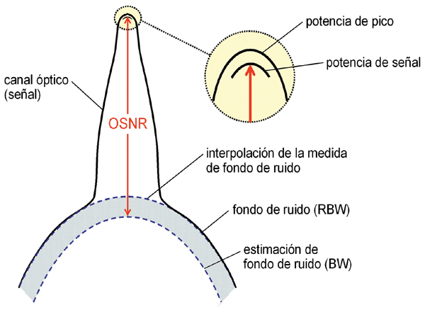 The resolution bandwidth must be chosen large enough to encompass the modulated signal. Under these conditions, the peak channel power value will include the total signal power plus the background noise level. The signal power value S (linear) is then obtained by subtracting the noise level from this peak value. To determine the noise level, both sides of the channel must be scanned at a distance large enough so that the background noise is not affected by the signal's skirts. The noise value can then be obtained by quadratic interpolation, as shown in Figure 2 (dashed line).
'
Since the traces were obtained with a specific resolution bandwidth, the values must be corrected for the equivalent bandwidth.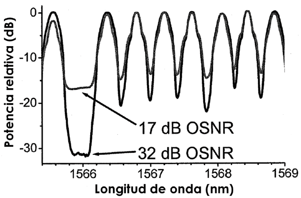 This calculation simply involves multiplying the (linear) OSNR value measured for a bandwidth RBW by the factor RBW/BW, where BW refers to the equivalent noise bandwidth (typically the channel bandwidth).
The accuracy obtained with this measurement procedure is very good. However, in the case of DWDM networks where the spacing between channels is quite small, the measurement becomes problematic. Figure 3 shows the optical spectrum of several DWDM channels with RZ modulation at 10 Gbit/s and a standardized ITU spacing of 50 GHz (0.4 nm). Note that there is very little spectral space between channels for monitoring. This means that, when the OSNR is high, the noise level measured near 1566 nm, where one of the channels has been switched off, is very different from the minimum power level that appears between channels. In general, 10 Gbit/s signals require a minimum channel spacing of 100 GHz for satisfactory OSNR monitoring results. Additionally, the fact that channels pass through an OADM or OXC also affects OSNR measurements, as the noise background is impacted by the response of the optical filters, and the channels also change wavelength. Consequently, adjacent channels may have traveled different paths through the network and have different noise levels. Thus, not only is a minimum channel spacing necessary, but sufficient spectrum is also required to estimate the two independent noise levels.
Finally, the Optical Rejection Ratio (ORR) of an OSA determines its ability to measure small signals near a peak. It is defined as the ratio of the power measured at a certain distance from the peak to the power at the peak of the OSA filter for a narrow-bandwidth input signal (equivalent delta function of linewidth much smaller than RBW). OSA manufacturers specify this parameter at 0.1, 0.2, and 0.4 nm from the peak. As stated in IEC 61280-2-9, an ORR at least 10 dB higher than the maximum OSNR value to be measured is required. Thus, to measure, for example, an OSNR of 25 dB at 0.2 nm of a channel (equivalent to 25 GHz at 1550 nm), an instrument with an ORR of at least 35 GHz is required, which would ensure a measurement inaccuracy of less than 0.42 dB. As an example, Figure 4 shows the error made in the OSNR measurement when using an OSA with a limited ORR value.
Other OSNR Measurement Techniques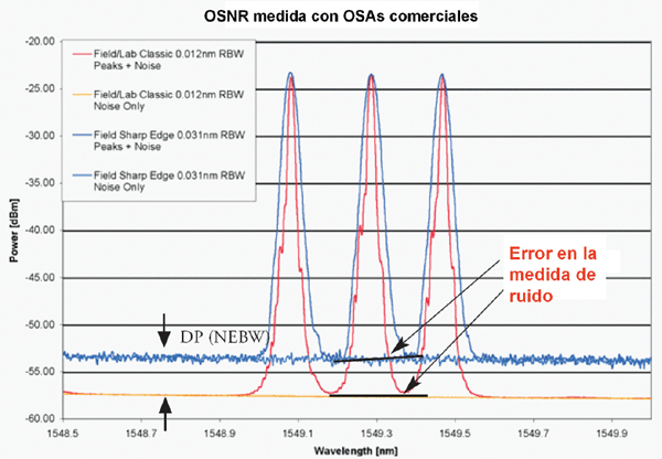 Besides OSA-based OSNR measurement, other techniques exist that allow for measuring the noise level within the optical channel itself. The difficulty in this case lies in discriminating noise from the signal, especially since the data signal is random and often appears as noise. To avoid this, one technique is based on using the polarization of the optical signal. In general, an optical signal will have a well-defined polarization state, while noise will be depolarized. Therefore, the polarization extinction ratio is a measure of OSNR. However, unfortunately, optical signals undergo polarization changes in fiber links due to PMD, which must be compensated for to make the technique valid.
'
Another technique for intra-channel OSNR measurement is based on capturing the amplitude spectrum of the data and monitoring specific areas of that spectrum where the signal is absent. This involves monitoring at low frequencies, high frequencies, or at specific nulls in the spectrum. Low-frequency monitoring, however, is affected by low-frequency noise tails, pattern-dependent fluctuations, and cross-modulation effects of gain in optical amplifiers. Additionally, many noise sources (e.g., multipath interference or MPI) have a strong influence at low frequencies, leading to an overestimation of the noise measurement. Conversely, at high frequencies, this noise is masked by frequency-independent ASE noise (white noise). At these frequencies, measurements are more sensitive to dispersive effects that cause fading. In short, these methods complicate network fault management because they don't actually measure the noise carried by the signal, but rather extrapolate that noise to high or low frequencies. Optical subcarrier monitoring has also been used for the direct measurement of OSNR and its correlation with the electrical SNR at the receiver output. The advantage of this technique is that it allows for the actual monitoring of the data signal propagating through the network.
Finally, electronic spectral monitoring techniques based on measuring noise in the data spectrum are very promising for fault management applications, as they allow for the direct measurement of noise present in the data. Some of these techniques include SONET signal frame monitoring, homodyne signal cancellation, and narrowband RF analysis at half the clock frequency. In subsequent articles, we will analyze some of these techniques in more depth, allowing us to evaluate their characteristics and performance. It should be noted, however, that the most standard method for measuring OSNR is the one presented in this article, which is implemented by the vast majority of optical spectrum analyzers on the market.
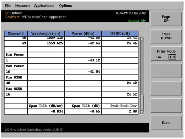
As an example, Figure 5 shows a results screen from one of these analyzers, where the OSNR measurements for two of the WDM channels can be observed.
Reference documents
IEC 61280-2-7: “Fiber-optic communication subsystem test procedures – Part 2-7: Data analysis of bit error ratio versus received power for digital fiber-optic systems”.
IEC 61280-2-9: “Fiber-optic communication subsystem test procedures – Part 2-9: Digital systems – Optical signal-to-noise ratio measurement for dense wavelength-division multiplexed systems.
Francisco Ramos Pascual. PhD in Telecommunications Engineering.
Full Professor at the Polytechnic University of Valencia.