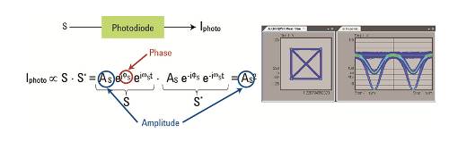
 OOK (on/off keying) modulation allows us to detect the signal with just a photodiode, which converts the optical power into an electrical current (IPhoto). The photocurrent IPhoto created by the photodiode is directly proportional to the product of the optical signal S and its complex conjugate S*. In the equation in Figure 1, we can see that the result only contains the amplitude AS. IPhoto provides no information about either the angular frequency ωs or the phase Φs. Therefore, a direct and unambiguous correspondence cannot be established between the QPSK modulation signal in the time domain on the right and the IQ diagram on the left. It can only be stated that the lower curve passing through zero represents the diagonal transitions between the four points of the constellation, and that the central curve represents the transitions that fall outside of it. The flat signal passing through 1 represents the cases where the phase does not change, that is, where one symbol is followed by the same symbol.
To unambiguously identify symbol transitions, we must look for more sophisticated methods that allow us to detect the complete electric field, including phase information.
To further complicate matters, current optical communication systems operate at wavelengths in the near-infrared region, for example, at 1550 nm, which corresponds to a frequency close to 200 THz. Therefore, changes in the electric field over time and space are several orders of magnitude too fast to be processed by available electronic devices, which operate in the MHz to GHz range.
 A local oscillator can help us.
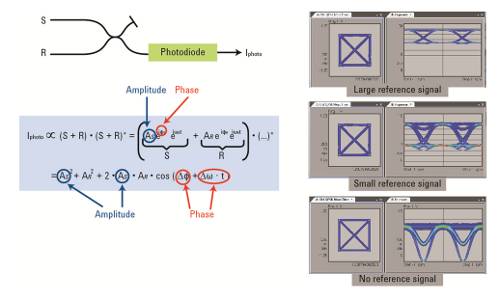
The key to solving both problems lies in measuring not only the absolute phase but also the phase relative to a known reference signal. Figure 2 shows the basic detection setup: the ideally monochromatic laser that generates the reference signal R is usually called a “local oscillator.”
The signal of interest S and the reference signal R are superimposed in an optical combiner and detected by the photodiode. Consequently, IPhoto is proportional to the product of the sum of both signals (R+S) and their complex conjugate (R+S)*. The equation in Figure 2 indicates that the result includes the phase difference ΔΦ = ΦS - ΦR and the frequency difference Δω = ωS - ωR. From ΔΦ, we can deduce the evolution of ΦS over time.
A reference frequency ωR close to ωS is chosen so that Δω is small enough to be processed electronically.
This phase-dependent value is called the "heterodyne value" because it results from combining the two signals.
There is also a value that contains the square of the amplitude, which is inconsequential as long as only the phase is modulated and the amplitude remains constant, as in the case of QPSK modulation.
At the bottom of Figure 2, we see the case without a reference signal mentioned earlier, where only the AS2 value is displayed.
When a large reference signal is added, compared to the signal itself, we essentially see that the heterodyne value shifts AR2 upwards. It would be interesting to be able to obtain the heterodyne value without this shift.
 Suppression of Phase-Independent Values with a Balanced Receiver.
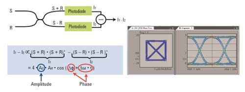
As shown in Figure 3, we can suppress the remaining phase-independent values with a balanced receiver. In this case, the signal we want to detect, S, and the reference signal, R, are summed in one branch and subtracted in the second branch of a 2x2 optical combiner (which can be a fiber optic or free-space coupler). A photodiode detects each of the resulting signals. The difference between the two photocurrents is then used. In the equation, also shown in Figure 3, we can see that the other values have been canceled, leaving only the heterodyne value.
Furthermore, balanced detection offers another advantage: the net photocurrent has been doubled.
 Application of the concept to the IQ plane: the IQ demodulator.
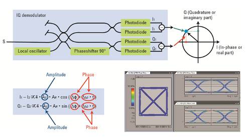
To capture both amplitude and phase, a coherent receiver should provide the in-phase (I) and quadrature (Q) components as two separate output signals. This requires a second balanced detector. A single local oscillator provides the reference signal for both detectors, but the phase must be shifted by π/2 to obtain the Q component. Figure 4 illustrates the complete setup, called the “IQ demodulator,” for a QPSK modulated signal.
This configuration only works for coherent signals that are not polarization-division multiplexed. Furthermore, the signal is only combined with the local oscillator component that has the same polarization state as the detector.
 Extending the Concept to Dual Polarization
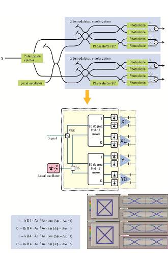
In the case of dual polarization, we need to further develop the demodulator concept. The basic principle remains the same: after a polarization splitter, we now have two IQ demodulators, one for the xy polarization and the other for the y polarization. A single local oscillator is used to provide reference signals for all branches.
The block diagram can be seen in Figure 5. As we can see, there are four output signals to resolve the I and Q coordinates, one for each polarization direction. In the equations, the upper indices h and v reflect the horizontal and vertical polarization state of the signal relative to the receiver's polarization reference frame. This architecture with multiple polarizations also ensures that the entire signal is combined with the local oscillator, regardless of the polarization state at the input. Therefore, its use is common even when the signal does not use dual polarization.
So far, we have seen receivers with a local oscillator of a frequency ωR that is different from the frequency of the signal ωS. These receivers are called “heterodyne receivers”.
In homodyne receivers, the local oscillator has the same frequency as the carrier signal. They have the advantage that the values mentioned above no longer depend on the frequency.
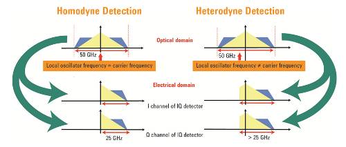 Figure 6 quantifies the electrical bandwidth required for both homodyne and heterodyne receivers. For homodyne detection, where the local oscillator operates at the same frequency as the signal itself, half the optical bandwidth of the signal is required. In the case of a heterodyne receiver, the electrical bandwidth requirement increases as the frequency offset between the local oscillator and the signal increases.
Using a Delayed Copy of the Signal as a Reference: Delay-Line Interferometers.
After what we have seen so far, it seems that using a local oscillator is indispensable for capturing phase information. What would happen if we superimposed the signal with a copy of itself? This would also allow us to obtain a reference signal where ωR = ωS.
One might think that this approach is not very promising, because it is not clear that this method allows us to obtain additional information about the phase. However, this self-homodyne approach is useful because what we are interested in is detecting the phase shift over time. Therefore, if we split the signal in two and superimpose the signal with the delayed copy as a reference signal, we will obtain information about the phase shifts.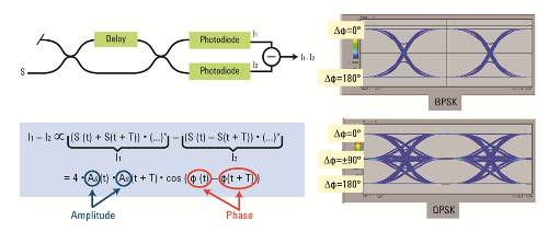 The advantage of this measurement method is that it is not subject to inaccuracies due to slow fluctuations (compared to the symbol rate) in the frequency of an external local oscillator or the carrier laser.
This type of receiver configuration is called a “delay-line interferometer.” Figure 7 shows a delay line interferometer with the signal S(t) and the signal S(t+T) delayed by T.
This equation indicates that the result depends on the phase difference between the original signal and its delayed copy. Due to the periodicity of this function, only phase differences between 0 and π can be unambiguously identified, and only for delays T that are approximately an integer multiple of the carrier period, 2π/ωS. This is sufficient for BPSK modulation. However, for phase capture in QPSK and higher-magnitude modulation schemes, we must add another phase-delay line interferometer, offset by π/2 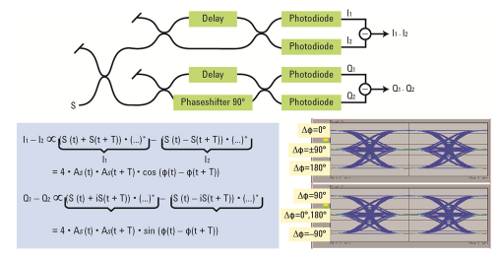 relative to the other, in order to cover the full phase range from 0 to 2π.
Figure 8 shows the configuration with an additional phase-delay line interferometer to receive the two independent components I and Q. Q1-Q2 is also measured, while I1-I2 remains unchanged.
Like heterodyne receivers, the delay-line interferometer can also be extended to perform polarization-sensitive measurements.
With a delay-line interferometer, we don't need an external local oscillator and therefore don't have to worry about the phase noise introduced by the oscillator. Furthermore, we require less signal processing. However, this approach has drawbacks that might lead us to choose a heterodyne receiver.
First, to measure phase changes over time using a delay-line interferometer without data capture/clocking (CDR), the delay and sampling period must be much smaller than the symbol period. Currently, symbol rates have reached a level that can make this condition extremely difficult to meet. Additionally, for low-power signals, the measurement sensitivity is reduced, since the reference signal is also low-power and is affected by noise accumulated in the transmission link. For implementations using a sampling technique, the measurement time increases, and a trigger is required. In summary, homodyne receivers are not very flexible.
Up to now, we have focused exclusively on time-domain detection techniques. However, we can also detect the frequency spectrum and make inferences from it by applying the Fourier transform to the time-domain signal.
Frequency Domain Detection:
To capture a complex modulated optical signal from its spectrum, we must measure the complex spectrum, that is, the spectrum containing both amplitude and phase information.
This can be accomplished using a complex spectrum analyzer that separates the different optical frequency components with a dispersive element. All frequency bands can be detected simultaneously using multiple detectors or sequentially with a narrow-band scanning optical filter and a single detector.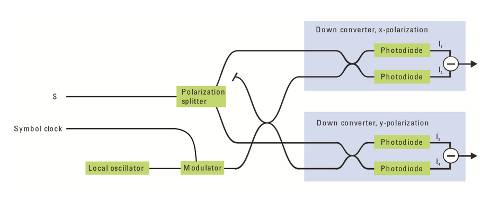 To capture the phase and amplitude, we again use a local oscillator to provide the reference signal. To capture both components, we need a source that emits two optical frequencies.
Figure 9 shows the complete setup required to measure the polarization-resolved complex spectrum.
The major advantage of frequency domain detection is its virtually unlimited bandwidth, which translates into unlimited time resolution. The bandwidth depends on the sweep range of the local oscillator to achieve bandwidths in the THz range with today's adjustable external cavity lasers. The other major advantage is that we don't need a high-speed receiver.
On the other hand, it also has significant drawbacks.
For example, it can only be applied to periodic signals, since these generate the necessary discrete spectral peaks. Furthermore, this option requires a symbol or pattern clock. The accuracy of the captured time-domain signal depends directly on the spectral resolution, which determines the number of sidebands that can be resolved. The spectral resolution achievable today limits the pattern length to a few tens of symbols.
These factors, along with the fact that this method doesn't provide real-time results, make frequency-domain detection unsuitable for network receivers. In fact, we would have to dedicate considerable time to measurements, in addition to creating a rather complex measurement setup and signal processing.
Finally, in frequency detection, all non-periodic effects are averaged out. The same applies to polarization mode dispersion (PMD), which, therefore, cannot be compensated for.
Preferences:
Autohomodyne configurations require little signal processing and are the least sensitive to phase noise. However, they are not very flexible, only operating close to the design symbol rate and are less sensitive than heterodyne implementations.
Time-domain detection methods using heterodynes offer the greatest flexibility. Unlike frequency-domain detection, they can be used for real-time detection. Therefore, they can be used on active signals in data networks. Equivalent-time sampling only works with repetitive signals of a limited length, for example, in test and measurement situations.
With real-time sampling, we can reconstruct the entire signal in all domains without limitations regarding the modulation format. We also do not have to deal with limitations regarding signal length with time-domain detection using heterodynes. Polarization mode dispersion (PMD) and chromatic dispersion (CD) can be compensated for during signal processing. In this case, the only limiting factor on performance is signal processing.
At the same time, we must be aware that this approach requires high-speed, four-channel equipment, such as a high-performance real-time digitizer with very low jitter and noise and a high effective bit number (ENOB) across the entire frequency range.
This covers the basics of receiver construction. In the next installment of this series, we'll examine the details of a real-time sampling setup in the time domain.
References
1 Block diagram extracted from “OIF Implementation Agreement for Integrated Dual Polarization Intradyne Coherent Receivers”
The remaining figures in this article are contributions from Oliver Funke, Bernd Nebendahl and Bogdan Szafraniec.
Author: Stephanie Michel, Keysight Technologies