 At speeds of 40 Gbit/s and above, it is well known that chromatic dispersion in the fiber limits the system's range to a few kilometers, necessitating the use of dispersion compensation techniques. However, in the presence of chirp, the degradation caused by dispersion in the optical pulses is generally even worse. More specifically, there is greater pulse broadening and interference between symbols, leading to a power penalty. Additionally, chirp also causes spectral broadening of the channels, thus limiting the available bandwidth. Therefore, it is important to have tools to measure and characterize the chirp levels of optical transmitters. Likewise, it is crucial to understand the causes of the phenomenon and to have a mathematical model that allows observation of the influence of the device's main parameters. Below, we will briefly describe some basic principles of chirp, both in the case of lasers and external modulators. The following article will present some of the main measurement techniques used for the characterization of the chirp of optical transmitters, as well as some examples of laboratory instrumentation.
Chirp Model.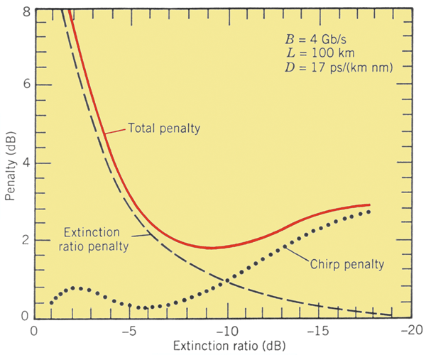 Before examining in detail the chirp generated in different types of optical transmitters, which typically has varying characteristics, it's helpful to begin with a definition of the phenomenon. Chirp can be defined as a residual and unwanted frequency modulation at the output of the optical transmitter that is strongly dependent on intensity modulation. For this reason, chirp is only generated in the device to which the modulating signal is applied, and it should not be confused with phase or frequency noise that affects the linewidth of lasers (Lorentzian frequency spectrum). Chirp can usually be decomposed into two components: transient chirp and adiabatic chirp. Transient chirp occurs during the rising and falling edges of the pulses; that is, it is proportional to the temporal variations of the optical power (modulating signal). In contrast, adiabatic chirp depends on the signal level, and therefore manifests as a frequency shift of the carrier between low and high levels. Expressed in an equation, the variations in carrier frequency due to chirp can be expressed as:
 where P(t) refers to the optical power of the signal. As can be seen in the equation above, the frequency variation (chirp) can be modeled as the sum of a phase-shift term (transient chirp) and a frequency-shift term (adiabatic chirp). Thus, an abrupt phase shift implies a frequency transient. The proportionality constants depend on physical parameters of the device, which we will discuss below.
Chirp in lasers.
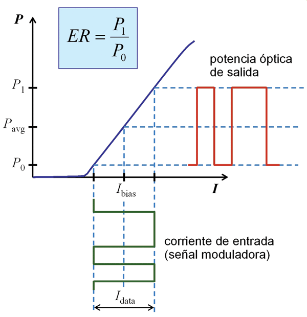
Lasers under direct modulation represent a low-cost option for short-range systems, although they should not be used in long-distance or high-speed systems due to the high levels of chirp that typically characterize them. For data signal transmission, the laser is biased with a direct current, Ibias, onto which the modulating signal, Idata, is applied. The average output power, Pavg, and the extinction ratio, ER, are adjusted by the amplitudes of these two current signals, as schematically represented in Figure 1. Generally, lasers produce more chirp as the extinction ratio increases, so there is a trade-off between the power penalties due to chirp and extinction ratio (signal-to-noise ratio). This can be observed in the graph in Figure 2.
The equation that characterizes the chirp of a laser under direct modulation is:
 where 'a' is known as the line broadening factor. The first term is the transient chirp, while the second and third refer to the adiabatic chirp. The transient chirp produces phase shifts of opposite sign for the rising and falling edges of the data signal pulses, these being inversely proportional to the duration of these edges (proportional to the slope or time derivative). In turn, the situation is complicated by the fact that these phase and laser gain jumps excite the device's natural resonance: relaxation oscillations. Then, until the laser stabilizes again,
  a significant energy loss occurs during this transient. Once stabilized, the new output power level has an associated frequency shift that corresponds to the second term of the previous equation (adiabatic chirp). Finally, the third term of the equation is due to spontaneously emitted photons.
Figure 3 shows an example of measuring the chirp levels of a DFB laser. As can be seen in the figure, there are significant levels of transient and adiabatic chirp. Transitions between high and low levels excite the device's relaxation oscillations, causing fluctuations in both the intensity and frequency of the optical signal. In fact, the frequency fluctuations (chirp) extend to a range of approximately 8 GHz. It is therefore clear that techniques are needed to reduce chirp levels in direct modulation optical transmitters.
Chirp in External Modulators
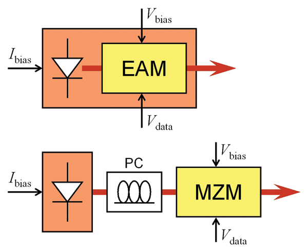
To limit the chirp levels of lasers under direct modulation, the use of external modulators was proposed (Figure 4). In theory, when the modulation process takes place outside the laser cavity, there is no adiabatic chirp. 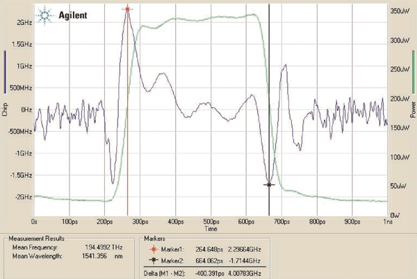 The constant-frequency carrier generated by the laser only has its amplitude and phase modified as it passes through the modulation section. In practice, however, optical reflections, thermal interactions, or parasitic packing effects can lead to adiabatic characteristics.
One of the most interesting options for external modulation is the electroabsorption modulator (EAM). Since they can be integrated with the laser on the same chip, transmitters can be manufactured at a reasonable cost. In this case, the modulating signal is applied directly to the EAM, usually represented as an electrical voltage signal. This electrical voltage controls the absorption of the waveguide (insertion losses), thus modulating the optical carrier generated by the laser. In this type of transmitter, performance is primarily determined by the transient chirp of the modulator, completely eliminating fluctuations due to laser relaxation oscillations. As an example, Figure 5 shows chirp measurements of an EAM-based optical transmitter. It can be observed that the chirp appears only during the rising and falling edges of the pulses, when the dP/dt term dominates.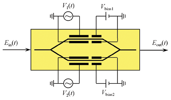 Alternatively, a Mach-Zehnder modulator can also be used for intensity modulation. In this case, the modulator is packaged separately, and the optical polarization at its input must be carefully controlled. This type of modulator is based on an interferometric structure made of a crystalline material such as lithium niobate (LiNbO3). The input optical signal is split into two branches where it is differentially phase-modulated by electric fields generated by two data signals (Pockels effect). Subsequently, these signals are recombined at the output, resulting in PM-IM conversion. Figure 6 shows the modulation scheme. The bias signals Vbias1 and Vbias2 are used to set the operating point of the modulator, which is characterized by a sinusoidal transfer function VP. The chirp value is given by the following expression:
where it can be observed that it can be eliminated if V1 = Vdata/2 and V2 = -Vdata/2.
Figure 7 shows chirp measurements for a Mach-Zehnder modulator with NRZ signals, clearly reflecting the low chirp levels that can be achieved: approximately 300 MHz peak-to-peak.
RZ modulation with chirp.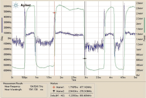 Despite the negative effects of chirp in optical transmitters, there are also situations where its presence is advantageous. This is the case with RZ signal transmission, where by appropriately adjusting the transmitter's chirp level, a reduced influence of chromatic dispersion can be achieved. Considering standard fiber in the third window and negative chirp values, it can be observed that the RZ pulses undergo initial compression. However, this effect only occurs over short distances, and as the fiber length increases, the results worsen compared to the situation without chirp.
Therefore, disregarding this latter point, chirp is generally a detrimental phenomenon that limits the performance of optical communication systems. This article has presented its fundamentals and characteristics, which depend on the type of optical transmitter used. In the next article, we will focus on measurement techniques and present some examples of commercially available equipment for these tasks.
Francisco Ramos Pascual. PhD in Telecommunications Engineering.
Full Professor at the Polytechnic University of Valencia.